How to replicate the performance of a popular mutual fund using common factors?

There is a large number of flagship investment funds within the U.S. investment industry with assets under management in the billions, reflecting their broad adoption by investors. The JP Morgan Global Asset Allocation Fund (JPM GAA) for instance is one these funds with asset under management of more than 2.8 billions USD.

That fund aims at maximizing total return over the long term and is for the most part unconstrained globally nor by asset class as it takes positions across global markets in equities, bonds as well as alternative assets. (See details https://am.jpmorgan.com/us/en/asset-management/adv/products/jpmorgan-global-allocation-fund-a-48121l734). It charges a bit more than 1% and has been around for about 15 years. The fees appear to fall within the higher bound of the range for select top actively managed funds. Thus, let’s dissect how the fund is designed especially its exposure to some main asset classes and the global value factor. We choose the S&P 500 as the market for equities, iShares Core US Aggregate Bond ETF (AGG) for the bonds, Vanguard Global Value Factor ETF (VVL) for the global value, the Dow Jones Commodity index for the commodity asset class, and the US dollar index for the US dollar.

Then we run a multiple regression of the JPM fund on these asset classes/factors to determine the degree of exposure on these asset classes as follows:

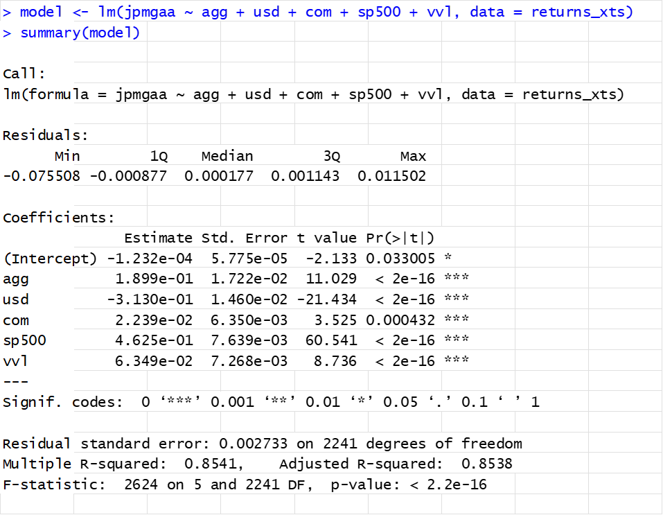
From these results we can observe that the 85% R- squared is very high, thus the returns on the JPM GAA Fund can be well explained by the assets classes/factors. JPM GAA Fund has not generated a positive alpha over the last 10 years. In fact, the alpha was negative over the last 9 years although this appears less significant than the other variables. The fund has been positively and significantly exposed to most of the asset classes with the S&P 500 contributing to the bulk of equity beta (0.46). The USD also explains a large part of the fund returns although negatively exposed (e.g when USD strengthens, the funds’ returns fall).

Now let’s visualize this graphically side by side in the following charts. In the first one (Fig1) we constructed a replication of JPM GAA returns using the asset classes /factor betas initially calculated over a 9 year period assuming the betas are static over the time frame.

Fig 1: Actual returns of JPM GAA vs replicated returns-daily returns-statics betas (2016-2025)

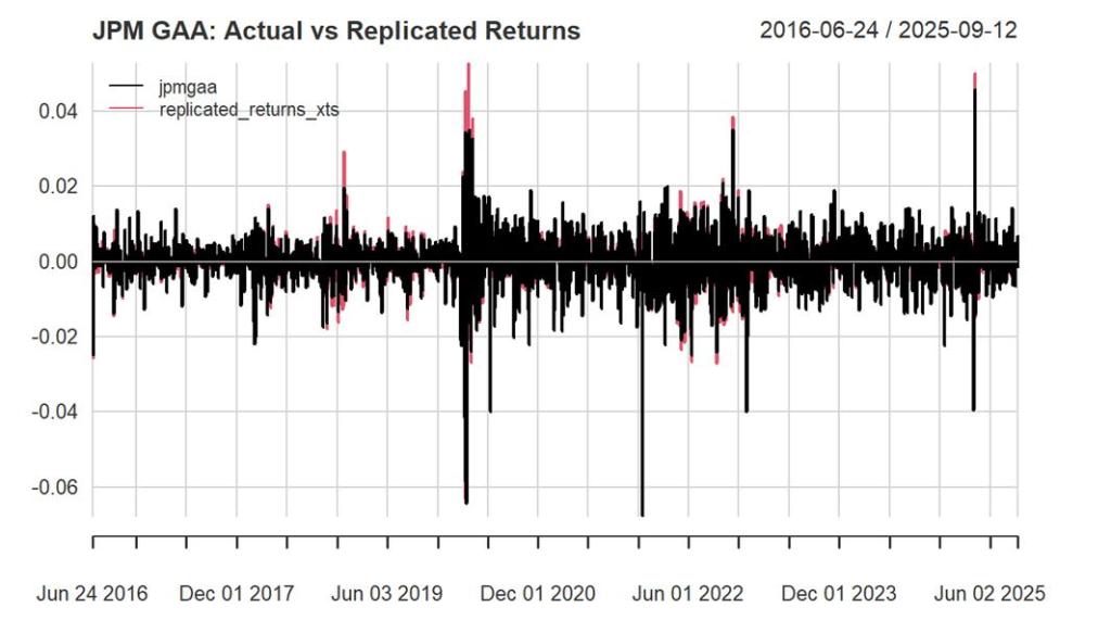
Sources: indices data from investing.com. returns calculation by author.

The fund and its replicated version using static betas/factors appear to follow each other tightly. To visualize this further Fig 2 plots their cumulative returns:

Fig 2

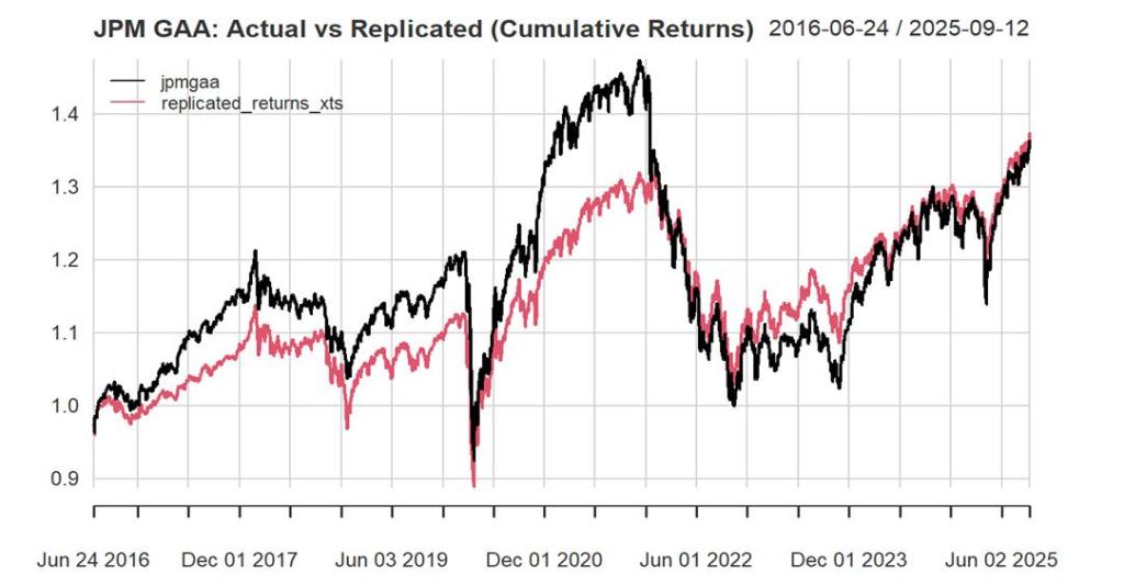
Sources: indices data from investing.com. returns calculation by author.

The replication has varied over the years with minimal gaps in some sub periods between the actual fund and its clone version but a bit bigger in others. One of the rationales relates to the calculation of betas as we assume them to be stable over the 9 years period. However, betas do fluctuate over time and in the following Fig 3 we use the rolling 60 days betas to build the replicated version of the actual funds.

Fig 3:

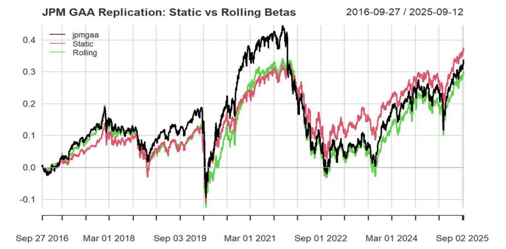
Sources: indices data from investing.com. returns calculation by author.

We observe a clear improvement when using rolling betas rather than static betas. Relative to the static specification, rolling betas substantially reduce the gaps between the cumulative returns of the actual fund and those of the replicated portfolio. While the replication is not perfect, the results suggest that investors who prefer not to take direct exposure to a popular fund can nonetheless achieve a close approximation of its performance. Through a careful selection and combination of asset classes or factors—ideally implemented using low-cost ETFs—investors can replicate much of the fund’s return profile while significantly reducing costs.